So last weekend, @encephalartos produced a graph of his tweets as extracted from his twitter archive, and thereby tempted me to spend the rest of my weekend and some extra time beyond figuring out how he did it. Turns out he used excel to break the timestamps and R to do the rest, but I didn't realise he used excel till I had spent hours figuring out time in R, so I present to you the entirely R way of doing it.
I like to use Rstudio for doing my R work. It's available for Linux, Windows and Mac so you've no excuse. Most of my R knowledge comes from workshops that Kevin O'Brien ran in Tog. If you're based in Dublin and want to hang with some R folk, the Dublin R group meets (ir)regularly around town.The Twitter archive is a great excuse to practise your R skills, as (depending on how much you tweet) it's a nice large dataset with results that will be interesting but not critical to the running of the world. You can download your archive by going to the settings page on twitter.com and at the very end, there's a button to click to request your archive. After a few minutes you get an email with a link to download the zipped archive that contains lots of delicious data. For these graphs, you only need the file tweets.csv which contains all your data as a handy flat file, where columns are separated by commas.
Getting the archive ready to graph
Importing your archive in Rstudio is really easy. Go to Tools>Import Dataset and follow the instructions (or you could look up a tutorial how to do it the proper R way, but why have an IDE if you don't use it :) ). The default settings should cover the tweets.csv but double check that it looks right in the preview pane.
The timestamps column is what's interesting to us today. It's formatted in ISO 8601 format, but Rstudio will have imported it as a character rather than a date, so we have to do some quick conversions.
You will also need to install/load the relevant libraries for the date handling and graphing.
install.packages("ggplot2")

install.packages("scales")

install.packages("lubridate")

#You only need to install once, but you need to load with library() every session.
library(ggplot2)
library(scales)
library(lubridate)
Convert the timestamp to POSIXct format using as.POSIXct() and put it in a new column (I don't like overwriting old columns).
tweets$posix_timestamp <- as.POSIXct(strptime(tweets$timestamp, '%Y-%m-%d %H:%M:%S'))
If you run data.class(posix_timestamp) it should return "POSIXct", confirming the data translation worked. Incidentally, when I looked at my new posix_timestamp column, I saw that it ended in GMT and IST depending on the time of year, it would seem IST is Irish Standard Time, which is equivalent to BST (British Summer Time). I think the conversion to IST might be due to my system settings being for Ireland.
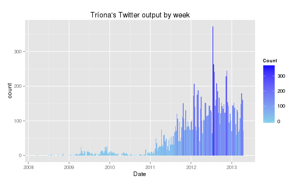
Graphing tweets by week
Once you have the dates converted to POSIX format you're pretty much there, you just need to generate the graph!
ggplot(tweets, aes(x=posix_timestamp)) + geom_histogram(binwidth = 60*60*24*7, aes(fill = ..count..)) +scale_fill_gradient("Count", low = "skyblue", high = "blue") + xlab("Date") + ggtitle("Tríona's Twitter output by week")
The natural bins for POSIXct objects are 1 second, so to get week-long bars, you have to multiply them up. The start of the "week" is presumably the start day of the archive itself, I need to get around to figuring that out.
You can play around with the binwidth to get days or years as you fancy. Likewise you can change the colours and titles.
In Rstudio, you can export your graph by clicking on the little "export" button over where the graph appeared. I like to export and .png but you can make your own choices about your preferred image type.
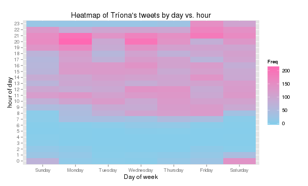
Graphing hours vs. weeks
Now that the time is in a POSIX friendly format from earlier, it's easy to extract parts of the date using the Lubridate package we installed.
tweets$day_of_week <- abbr="FALSE)<br" label="TRUE," wday(tweets$posix_timestamp,>
tweets$hour_of_day <- hour(tweets$posix_timestamp)
We then take these new columns and convert them into a table to make them easier to graph as their frequencies will be listed. A table can't be directly graphed, so we convert it into a dataframe and we can work on from there.
daytime <- table(tweets$hour_of_day, tweets$day_of_week)

dfdaytime <- as.data.frame(daytime)
dfdaytime should be return data frame rather than table when you run data.class(dfdaytime).
R will have renamed the columns when it created the table, with hour_of_day becoming Var1 and day_of_week becoming Var2. Frequency will be in a third column called Freq
Now that we have the new dataframe made, we can plot the graph!
ggplot(dfdaytime, aes(x=Var2, y=Var1, fill=Freq)) + geom_tile() + scale_fill_gradient(low = "skyblue", high = "hotpink") + ggtitle("Heatmap of Tríona's tweets by day vs. hour") + xlab("Day of week") + ylab ("hour of day")
As before, fiddling with the colours and labels of axes and graph title are easy. Choosing a colour that makes the data clearest is the hard part...
Further rambling
ggplot2 is a pretty powerful package in R for making graphs, and thanks to this bit of twitterage, I'm that bit closer to mastering it. Part of its power comes in the piecemeal assembly of the graphs (you spotted the +'s between each chunk of graph code), so after declaring what you want in the graph and the type of graph, you can start adding on other bit to en-fancy-fy the graph further.
The graphs include retweets, so I need to figure out the easiest way to sieve them out (about 25% of my tweets are retweets). I also need to figure out how to make the bins align with the start of the week. I should probably also reproduce the heatmap for the last year, so my supervisors can see I don't spend my entire work day tweeting :D